Finance 3.0 - The AI Revolution

Finance 3.0 - The AI revolution

In 2012, there were only 12 active hedge funds utilizing some form of AI in their trading program according to Preqin, a world renowned hedge fund database. In 2018, there were more than 305 hedge funds with aggregated assets surpassing 17 billion. Over a 6 year span and after seeing positive performance by machine learning models, the increase was over 2000% and the growth of hedge funds using AI in 2019 was about 60%. This is why Adaptive Alph believes it’s important to explain how machine learning, a subset of AI, is paving the way for investment professionals to enter the world of finance 3.0. For many years now, advanced statistical techniques has proven to outperform human decision making in narrow fields such as language translation, Google search and cancer detection. Advanced recursive algorithms now also provide investors with an uncorrelated return stream to their traditional equity and fixed income portfolio.

Game of GO

GO - the ultimate machine learning problem

Does the above picture look familiar to you? If you guessed GO – then you were correct! Current intellectuals demonstrate their intelligence by playing this ancient Chinese board game. It was also popular among past Chinese emperors, as it was said to demonstrate a general’s skill in “the art of war”. This as the complexity of the game requires deep thought to come up with a strategy and require its players to continuously tweak their strategy to defeat their opponent. Despite GO’s complexity, the game also provides an excellent obstacle for a machine learning engineer. GO is a game with a predefined set of rules, is limited to two players and in total there are more possible moves than there are stars in the sky. The ultimate goal for many of our best AI engineers is to create intelligent artificial beings. We must therefore define intelligence, which Max Tegmark does in his book, Life 3.0, as the ability to solve complex problems. Given the natural complexity of GO and the ultimate goal of AI engineers, scientists all over the world raced to build AI machines that could beat the best human GO players. In the game, each player takes a turn to place a piece at the intersections. The player that conquers > 50% of the board wins. GO is vastly more complex than chess because after two moves there are close to 130,000 possible moves compared to chess in which there are 400. Predefining a strategy for GO therefore requires rigorous number crunching, which is a perfect problem for a strong computer and an impossible problem for a human brain. If you ask the best GO players why they made a particular move they will often say it was intuitive as a result of the game’s complexity, but to play GO the computer can create an optimal strategy conditioned on the playing style of the opponent using statistics, probability theory and optimization; In other words, GO is a perfect problem to solve for a machine learning algorithm such as a deep neural network. In March 2016, scientists were successful in creating a computerized GO player as the AI, AlphaGo, beat the world’s number one GO player, Lee Seedol, in best out of 5 matches. Our question is then; If AI can be applied to a complex game like Go then why can’t it be applied to the markets?

Lee Sedol vs AlphaGO

Finance 1.0

Before diving into machine learning and finance 3.0, we must define the first two levels of finance. Adaptive Alph defines finance 1.0 as the investor’s ability to outperform the markets using a discretionary approach with limited use of computers. A finance 1.0 investor would be like Lee Sedol playing GO because it involves a theory and intuition driven approach, while Alpha GO or a finance 3.0 investor both use a data driven approach. Warren Buffet is a great example of a finance 1.0 investor because he is a stock picker. He obviously uses computers and does quantitative analysis of companies, but ultimately, he would make a discretionary decision to buy or sell the stock he analyzes. His theory is to find deep value stocks and he uses a cigar analogy as demonstration. He compares a cheap stock to a cigar that the market believes is burnt out, however, Warren knows that the cigar still has a couple of hits left. He then buys the stock at a low price and hopes to a make great return as the market starts hitting that cigar. You can call his cigar analogy the theory that motivates Warren to buy other companies.

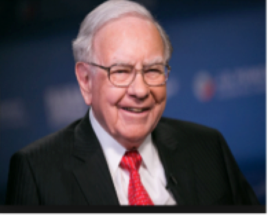
Warren Buffet

Finance 2.0

We then define a finance 2.0 investor as one using his ability to consistently beat the markets in a systematic fashion by combining human intuition with the number crunching power of computers. This finance 2.0 trading style is still theory driven like Warren’s finance 1.0 style, but it requires a deeper symbiosis with computers to generate returns. Jim Simons who is the CEO of the greatest hedge fund to ever exist, Rennesaince Technologies, is a great example because his fund runs multiple strategies all attacking the market utilizing a systematic quantitative approach. Rennesaince would not exist if it were not for the advances in computing power during the late 1990s (Thanks to Moore’s law, but that is another book). Quantitative hedge funds similar to Rennesaince build models based on patterns through number crunching large amounts of data from the past. A common misconception is that a quantitative investment strategy is a form of black box, but that is not really the case because these computer driven strategies are applying the same concepts as the finance 1.0 investors. The difference is that systematic investors predefine their trading strategy, which requires a great deal of deep thought. Prior to deploying a model, the systematic investors must account for volatility of the market, correlation between instruments being traded, correlation to other models in the trading system and political risks, just to name a few. The model must therefore have a built in risk management system, although most systematic systems typically have a panic button to prevent the model from trading if a black swan or any unforeseen macro event shows up in the data. As one might already have concluded, it is extremely difficult to predict the future so a systematic investor must rely on making data driven decisions based on patterns in the past that hopefully will continue into the future. One pattern that often emerges in financial instruments is strong up and down trends in price due to herding behavior by investors. Firms that take advantage of these trends are called trend-followers and they build highly quantitative models to forecast these trends. Sometimes it is also important to create a model that does not strongly outperform as the market will notice the utilization technique or edge and remove the advantage, however, important to note is that this ultimately makes markets more efficient. Adaptive Alph would argue that an exceptional yet mediocre model is most likely to outperform, as the model will make money while going unnoticed by other players in the market. Such a mediocre model extracts surplus, survives paradigm shifts and does not make the markets more efficient.

Jim Simons a legendary investor and a math genius

Now to the new part: Finance 3.0

Adaptive Alph defines a successful investor in finance 3.0 as one who provides the computer with an optimal framework of the game, which is the market for investment professionals, combined with the objective to achieve a high risk adjusted return. This is synonymous to the utilization definition of machine learning, which is the ability to automatically learn and improve from available data to achieve the set objective, instead of following static, explicitly programmed instructions much like the quantitative approach in finance 2.0. In the end, there are two major differences between the finance 2.0 and finance 3.0 technique. Can anybody guess? Okay let Adaptive Alph explain – the model under finance 3.0 is recursive and can find complex patterns in the market that does not fly under a human behavioral theory banner such as herding, gambler’s fallacy and loss aversion. In other words, in finance 3.0 dynamics the computer creates its own intuition through carefully analyzing data to make forecasts based on unexplainable complex patterns and when making a forecast error tweaks the prediction like an investor using a finance 1.0 value approach would do if they bought a company ending up being a burnt out cigar. The machine learning model therefore has the ability to update itself to make optimal forecasts even when paradigm shifts in the economy takes place. It is true that the rules of the market are more complex than GO, but the objective is the same - to win. There are basically two components of a trade, its direction (buy or sell) and its position size. What favors an AI model in the market versus an AI in the game of GO is that financial models only need to be correct 53% of the time to make money! Also, when the model generates a strong signal to buy an instrument then the position size in that instrument is larger than the position size in an instrument with a weaker signal ceteris paribus and some prediction systems can therefore have a hit ratio below 50% and still be successful. To create a successful machine learning algorithm the following 3 parts are needed, first, large amounts of data, second, high computing power to process the data and finally you need accurate, complete, consistent and timely data. Combine this with talented researchers and boom you have created robot Einstein. Below is an explanation of support vector regression, a machine learning technique, hopefully not described in to technical terms.

Support Vector Regression

Supervised and unsupervised learning are the two types of algorithmic approaches that exist within machine learning. Support vector regression (SVR) falls under the supervised approach, which means that the model developer defines the input variables that are used to forecast the output variable in the model. For example, if the output is a directional signal of the S&P 500 price, recent price volatility and momentum could be used as the input variables for the forecast (the variability of price and the change in speed of price). Unlike traditional learning models, which try to minimize the errors of making a mistake, SVRs are structural risk models that have lower risk of making errors with future data. In a traditional learning model, like OLS multiple regression taught in your typical statistics 101 course, the error to minimize is the actual value - forecasted value and when that is achieved the model is optimal. However, one could expect the prediction error to be large if price volatility and momentum was used on data from the period 1990-2009 to train the regression model to forecast the direction of the price of S&P 500 in 2010. This as the relationship between the input and output is non-stationary (changes over time) and thus it is highly probable that the empirical risk model is overfitted to the historical training data shown in the right graph below. However, in machine learning algorithms such as SVRs two extra items, the concept of a margin and the regularization variable, are added to the regression to prevent the model from overfitting to the training data and therefore decrease the risk of making future forecast errors.

Empirical risk models tend to extrapolate the past to create an identical future

When these extra terms are added, the model developer achieves structural risk minimization rather than empirical risk minimization. The goal of SVR is then to find the optimal line (hyperplane) that fits the data points as close possible. The margin prevents overfitting to the data and the regularization variable prevents the regression line or hyperplane to change to quickly to outlier data points.

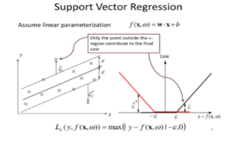
A two dimensional support vector regression to the left and a loss function graph to the right

The data points in finance represented by x in above graph are usually limited in nature to price, volatility and calendar data. As a visual experiment, one can think of the data points as a bunch of pennies on a table representing price data and the prediction line can be imagined as a magnet. The SVR would then place the magnet on the table to maximize the attraction to as many pennies as possible, which in other words is equal to minimizing the perpendicular distance among the data points. When you minimize the perpendicular distance you have a model that fits the data or attracts pennies in an optimal way and you can then make an optimal inference based on the underlying patterns in the data. The goal is to find a line/plane that does not deviate by more than the outer bounds represented by epsilon (ε). If observations start coming outside ε in the picture above, the model would update itself by fine tuning the weights on the regression coefficient inputs in a walk forward fashion. In other words, the model updates as new data is inputted to the model. Obviously, if there are rare extreme events the regularization term is used to control the model from deviating from the “normal”. In finance, quantitative models analyze noisy continuous price data and the dimensions are almost infinite and the more dimensions in the dataset, the more complex the dataset and therefore the more important the SVR technique becomes. In other words, SVRs scales in a nonelinnear fashion and it would be extremely difficult for a human to put the magnet in the perfect spot on the table if there are a billion pennies.

DONE!

1.

https://www.preqin.com/insights/blogs/the-rise-of-the-machines-ai-funds-are-outperforming-the-hedge-fund-benchmark/26411